Definition
Let p0, p1, p2, p3 be
quadratic polynomials in two variables u, v. This means each
pi is of the form
pi(u,v)=Au2+Buv+Cv2+Du+Ev+F
for constant coefficients A, B, C, D, E, F. The parametric plot
(x,y,z)=(p1/p0, p2/p0, p3/p0)
for some range of input values u, v, the image should be a
two-dimensional surface in (x,y,z)-space. It's called a Steiner
surface patch, but what does it look like? This web site lists all the
different geometric types of Steiner surfaces. Usually, graphing
polynomial quotients only gives a patch --- a part of the whole
surface. The mathematical setting for describing the entire surface is
projective geometry.
Background
The "real projective plane" is the set of lines through the origin
in real 3-dimensional space; when each of these lines is represented
by one point, the resulting set is, in an abstract way, a smooth,
two-dimensional surface. There are many ways to represent this surface
as a two-dimensional subset of three dimensional space, and some of
these representations were studied by J. Steiner. Here's some
background on the geometry of Steiner's images of the real projective
plane.
A convenient way to assign coordinates to the real projective plane
is to pick a coordinate system for real 3-space with axes labeled
u0, u1, u2, and denote by
[u0 : u1 : u2] the line equal to the
set of all scalar multiples of the non-zero ordered triple
(u0,u1,u2). So [1 : 2 : 3] denotes
the same line as [2 : 4 : 6], and another example is [0 : 1 : 0],
which is the u1-axis. This mathematical description of the
projective plane is called a "homogeneous coordinate system," and it
generalizes to any dimension: real projective n-space is the
set of lines through the origin in n+1 dimensions.
The starting point for our approach to Steiner surfaces is the Veronese variety, a smooth, 2-dimensional surface, given by embedding the projective plane into projective 5-space by the homogeneous parametric equations
[u0 : u1 : u2] --> [u02 : u12 : u22 : u1u2 : u0u2 : u0u1].
(Note that the map is well-defined! Changing the input vector by multiplying by a non-zero scalar gives an output vector also changed only by scalar multiplication.)
This surface can be projected into 4-space smoothly, but any
projection into three dimensional space must have singularities. Such
a projection is defined by multiplying the 1 by 6 vector with a 6 by 4
matrix, so composing the Veronese map with the projection matrix gives
four linear combinations pi of these six monomials. The
image of such a parametric map into projective 3-space is called a
Steiner surface; examples include the Roman surface and the Cross Cap
surface. The geometric properties of Steiner surfaces, including the
degree and the number and type of singularities, such as pinch points,
double lines, and triple points, depend on the projection from five
ambient dimensions to three.
A natural way to classify Steiner surfaces is to say that two are
equivalent if they are related by linear transformations of the domain
(the projective plane, [u0 : u1 :
u2]) and the range (projective 3-space, coordinates
[x0 : x1 : x2 :
x3]). A classification of Steiner surfaces was known in the
XIX century in the case where the coordinates and projective
transformations are allowed to be complex. A classification in the
real case has been studied in our paper:
A. Coffman, A. Schwartz, and C. Stanton, The algebra and geometry of Steiner and other quadratically parametrizable surfaces, Computer Aided Geometric Design (3) 13 (April 1996), 257-286.
- Updated comments on the
paper:


- CAGD article's ScienceDirect abstract (and full text link for some users)
A parametrization of a Steiner surface patch in a 3-dimensional
affine neighborhood by quadratic rational functions can be obtained
from the quadratic polynomials by "dehomogenizing": using two domain
variables u=u1/u0 and
v=u2/u0, and three range variables, so that
dividing by the first homogeneous coordinate transforms, for
example,
[x0 : x1 : x2 : x3] =
[p0 : p1 : p2 : p3] =
[u02+u12+u22
: u1u2 : u0u2 :
u0u1]
into the fractions
(x1/x0 , x2/x0 ,
x3/x0) = (x , y , z) =
(p1/p0 , p2/p0 ,
p3/p0) = (uv/(1+u2+v2) ,
v/(1+u2+v2) ,
u/(1+u2+v2)).
In fact, this description is just a fancy way to state the original
definition of a Steiner surface: the image of three rational functions
of two variables, where the numerators are any three quadratic
polynomials, and the denominators are equal quadratics. The 24 entries
in the projection matrix are exactly the coefficients appearing in the
quadratics. The (x,y,z) variables are the usual Cartesian coordinates
for three dimensions; this shows how real projective 3-space contains
the Cartesian 3-space, as the subset where x0 is
nonzero. This subset is called an "affine neighborhood," and the
subset defined by x0=0 is the "plane at infinity," where
the x1/x0, etc., fractions are undefined.
The following list of Steiner surfaces represents each equivalence
class from the classification theorem, and gives several different
ways to describe each object. Starting with a quadratic homogeneous
parametrization in [u0 : u1 : u2], a
homogeneous implicit equation can be derived. This procedure is called
"elimination of parameters," and I used the algebra
program Macaulay. Then, the inhomogeneous implicit equation
is given, in the affine coordinates x=x1/x0, y=
x2/x0, z=x3/x0. There are
also parametrizations by trigonometric or other functions, which are
more efficient for parametrizing the whole surface, instead of just a
patch.
Some of the parametric surfaces have self-intersections along line
segments, called double lines. When the parameters are eliminated to
get the implicit equation, there are some "extra solutions": points
which satisfy the implicit equation, but which do not appear as images
of the parametric maps. These extra solutions extend the line segments
to infinite lines, and appear as "whiskers" (or "umbrella handles")
sticking out of the surface. (In general, if a line meets a quartic at
more than four points, then the line must be contained completely
inside the quartic.) In the POV code, some of the whiskers have been
clipped off, and some are already invisible because the light rays
that reflect off the surface miss these lines entirely.
I've posted some code, which at least has worked for me, using a
Gateway 2000 E-3100 computer. The Maple code worked
with Maple V Release 4 Version
4.00b. The command with(plots); invokes the Maple
graphics package, and then the plot3d, display3d
and animate3d can be displayed in a new Maple window where
one can rotate, color, and otherwise manipulate the surfaces in
space.
The POV-Ray implementation was based on similar internet graphics
galleries, and was developed using POV-Ray™ Version
3.1a.watcom.win32. Click on the small picture to get a larger
picture. The code for the larger picture is available as
a .txt file. The POV program uses the affine implicit
equation of the surface, instead of the parametric plot used by
Maple.
I would be glad to hear about any use you find for this page,
including pictures you make and post to the WWW. I will also entertain
questions and suggestions. My email is CoffmanA (at) pfw.edu
--- you can acknowledge this resource by citing our CAGD paper or
linking to this
URL: http://users.pfw.edu/CoffmanA/steinersurface.html
--- as of Summer 2018, this replaces some now obsolete addresses at
IPFW and Chicago.
Equations and Graphics
1.
|
POV code
|
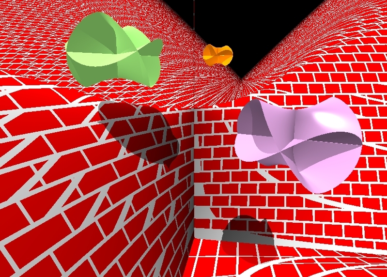
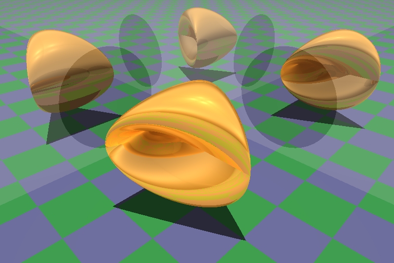
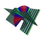
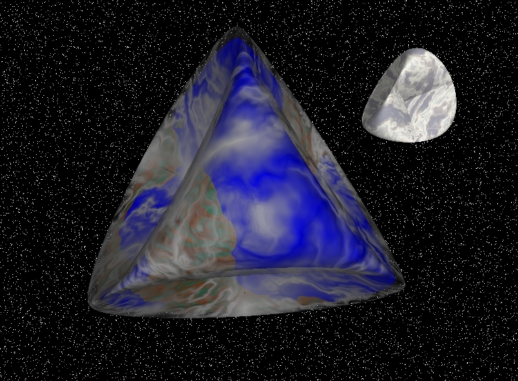
Steiner's Roman Surface. Three double lines, six pinch points, and a triple point. For a few more images, see my graphics gallery.
- homogeneous parametrization: [u02+u12+u22 : u1u2 : u0u2 : u0u1]
- homogeneous implicit: x12x22-x0x1x2x3+x12x32+x22x32
- affine implicit: x2y2+x2z2+y2z2-xyz = 0
- affine trig parametrization: x=r2sin(t)cos(t), y=rsin(t)(1-r2)(1/2), z=rcos(t)(1-r2)(1/2), 0<=r<=1, 0<=t<=2Pi.
- plot3d([r^2*sin(t)*cos(t), r*sin(t)*(1-r^2)^(1/2), r*cos(t)*(1-r^2)^(1/2)], r=0..1, t=0..2*Pi, numpoints=2500);
|
2.
|
POV code
|
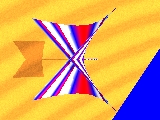
This surface can be transformed into Steiner's Roman Surface, by a complex change of coordinates (transforming x to ix and z to iz interchanges the Type 1 and 2 implicit equations, where i2=-1). It can also be transformed into the Type 3 Cross-cap by a complex transformation, but Types 1, 2, and 3 are not related by any real transformation. It has two real pinch points and three double lines meeting at a triple point, and, unlike the Roman or Cross Cap, is not compact in any affine neighborhood.
- homogeneous parametrization: [u02-u12+u22 : u1u2 : u0u2 : u0u1]
- homogeneous implicit: x12x22-x12x32+x22x32-x0x1x2x3
- affine implicit: x2y2-x2z2+y2z2-xyz = 0
- affine trig parametrization: (requires two components)
- x=rcos(t)(r2-1)(1/2), y=r2cos(t)sin(t), z=rsin(t)(r2-1)(1/2), r>=1, 0<=t<=2Pi,
- x=-rcos(t)(r2+1)(1/2), y=-r2cos(t)sin(t), z=-rsin(t)(r2+1)(1/2), r>=0, 0<=t<=2Pi.
- display3d({plot3d([r*cos(t)*(r^2-1)^(1/2), r^2*cos(t)*sin(t), r*sin(t)*(r^2-1)^(1/2)], r=1..1.5, t=0..2*Pi, numpoints=2500), plot3d([-r*cos(t)*(r^2+1)^(1/2), -r^2*cos(t)*sin(t), -r*sin(t)*(r^2+1)^(1/2)], r=0..1, t=0..2*Pi, numpoints=2500)});
|
POV code
|
The linear transformation which interchanges the x0 and x2 coordinates gives another view of the Type 2 surface, where two of the double lines are on the plane at infinity. The double line connecting the two real pinch points is still visible in this affine neighborhood. Planes containing this double line intersect the surface along parabolas, so this representation has been called a "parabolic Steiner surface."
- homogeneous parametrization: [u0u2 : u1u2 : u02-u12+u22 : u0u1]
- homogeneous implicit: x12x02-x12x32+x02x32-x2x1x0x3
- affine implicit: x2-x2z2+z2-xyz = 0
- affine trig parametrization: x=rcos(t), y=sec(t)csc(t)-r2cos(t)sin(t), z=rsin(t), r>=0, 0<=t<=2Pi.
- plot3d({[r*cos(t), sec(t)*csc(t)-r^2*cos(t)*sin(t), r*sin(t)], [r*cos(t+Pi/2), sec(t+Pi/2)*csc(t+Pi/2)-r^2*cos(t+Pi/2)*sin(t+Pi/2), r*sin(t+Pi/2)]}, r=-3..3, t=0.1..Pi/2-0.1);
|
3.
|
POV code
|
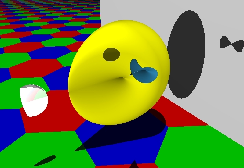
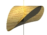
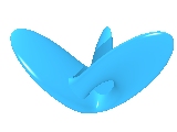
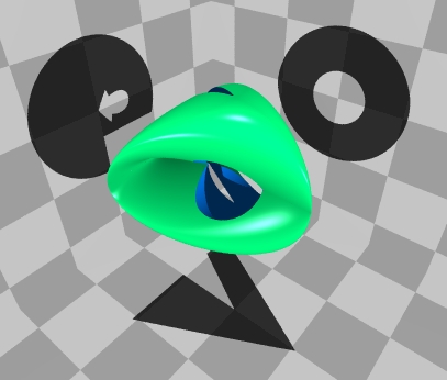
Steiner's Cross Cap. (equations from F. Apéry's book) One real double line is visible, but there are also two complex double lines, which would only be visible after a complex coordinate change, resulting in a Type 1 or 2 surface. There are two real pinch points, which curve in different directions (see the patches in the larger picture). It's also known as the Cross-Cap or Crosscap, and the pinch points are also called cross-cap singularities or Whitney singularities.
- homogeneous parametrization: [u02+u12+u22 : u1u2 : 2u0u1 : u02-u12]
- homogeneous implicit: 4x12(x12+x22+x32+x0x3)+x22(x22+x32-x02)
- affine implicit: 4x2(x2+y2+z2+z)+y2(y2+z2-1) = 0
- affine trig parametrization: x=rsin(t)(1-r2)(1/2), y=2rcos(t)(1-r2)(1/2), z=-1+r2+r2cos(t)2, 0<=r<=1, 0<=t<=2Pi.
- plot3d([r*sin(t)*(1-r^2)^(1/2), 2*r*cos(t)*(1-r^2)^(1/2), -1+r^2+r^2*cos(t)^2], r=0..1, t=0..2*Pi, numpoints=2500);
|
4.
|
POV code
|
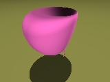
Two of the three double lines in the Type 2 surface here coincide, forming a "tacnodal" line, along which two neighborhoods of this noncompact surface appear to be tangent. This line contains one of the two pinch points, and the remaining double line connects the two pinch points.
- homogeneous parametrization: [u02-u12+u22 : u22-u12 : u1u2 : u0u1]
- homogeneous implicit: x02x22-2x0x1x22-x0x1x32+x12x22+x12x32-x34
- affine implicit: y2-2xy2-xz2+x2y2+x2z2-z4 = 0
- affine trig parametrization: (requires two components)
- x=1-r2cos(t)2, y=rsin(t)(r2-1)(1/2), z=rcos(t)(r2-1)(1/2), r>=1, 0<=t<=2Pi,
- x=1+r2cos(t)2, y=-rsin(t)(r2+1)(1/2), z=-rcos(t)(r2+1)(1/2), r>=0, 0<=t<=2Pi.
- display3d({plot3d([1-r^2*cos(t)^2, r*sin(t)*(r^2-1)^(1/2), r*cos(t)*(r^2-1)^(1/2)], r=1..2^(1/2), t=0..2*Pi, numpoints=2500), plot3d([1+r^2*cos(t)^2, -r*sin(t)*(r^2+1)^(1/2), -r*cos(t)*(r^2+1)^(1/2)], r=0..1, t=0..2*Pi, numpoints=2500)});
|
5.
|
POV code
|
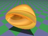
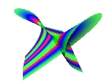
Two of the three double lines in Steiner's Roman Surface here coincide, forming a tacnodal line meeting the other double line in a "T" shape, and four singularities at the segment endpoints. It is related to the previous surface by complex but not real transformations.
- homogeneous parametrization: [u02+u12+u22 : 2u0u2 : 2u0u1 : u02-u12+u22]
- homogeneous implicit: x02x12-x02x22-2x0x12x3+x24+x12x32+x22x32
- affine implicit: x2(z-1)2+y2(y2+z2-1) = 0
- affine trig parametrization: x=2rcos(t)(1-r2)(1/2), y=2rsin(t)(1-r2)(1/2), z=1-2r2cos(t)2, 0<=r<=1, 0<=t<=2Pi.
- plot3d([2*r*cos(t)*(1-r^2)^(1/2), 2*r*sin(t)*(1-r^2)^(1/2), 1-2*r^2*cos(t)^2], r=0..1, t=0..2*Pi, numpoints=2500);
|
6.
|
POV code
|
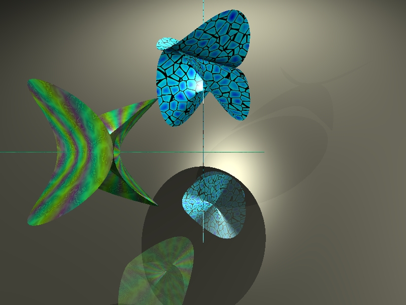
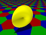
The three double lines of Steiner's Roman Surface coincide, forming an "oscnodal" line. I call this type the "Cross Cup," since it resembles the Cross Cap, but with the double line tangent to the surface.
- homogeneous parametrization: [u02+2u12+u22 : 2u12+u22 : u22+2u0u2 : u1u2+u0u1]
- homogeneous implicit:
x03x1-13/4x02x12+7/2x0x13-5/4x14+5/2x02x1x2-11/2x0x12x2 +3x13x2-1/4x02x22+5/2x0x1x22-5/2x12x22-1/2x0x23+x1x23-1/4x24 -2x02x32+5x0x1x32-3x12x32-3x0x2x32+4x1x2x32-x22x32-x34
- affine implicit:
-5/4x4+3x3y-5/2x2y2+xy3-1/4y4-3x2z2+4xyz2-y2z2-z4 +7/2x3-11/2x2y+5/2xy2-1/2y3+5xz2-3yz2-13/4x2+5/2xy -1/4y2-2z2+x = 0
- affine trig parametrization: x=1-r2+r2sin(t)2, y=r2sin(t)2+2r2sin(t)cos(t), z=((1-r2)/2)(1/2)r(sin(t)+cos(t)), 0<=r<=1, 0<=t<=2Pi.
- plot3d([1-r^2+r^2*sin(t)^2, r^2*sin(t)^2+2*r^2*sin(t)*cos(t), ((1-r^2)/2)^(1/2)*r*(sin(t)+cos(t))], r=0..1, t=0..2*Pi, numpoints=2500);
|
7.
|
POV code
|
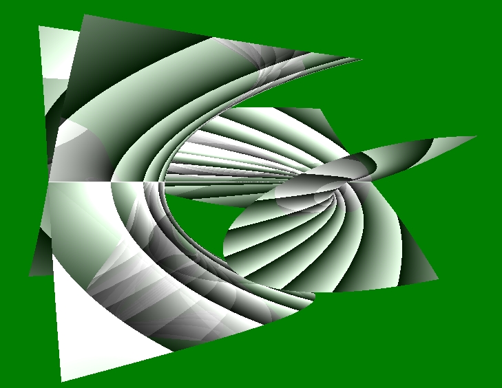
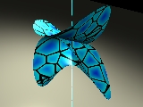
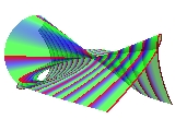
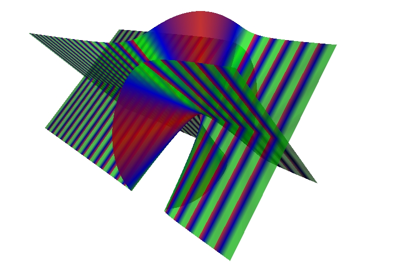
Quadratically parametrized surfaces can also have cubic implicit equations. The surfaces turn out to be ruled by lines. There are trigonometric parametrizations, but also convenient algebraic parametrizations. This cubic surface has a double line and no pinch points. It is sometimes called Zindler's conoid.
- homogeneous parametrization: [u12-u22 : u1u2 : u0u1 : u0u2]
- homogeneous implicit: x1x22-x0x2x3-x1x32
- affine implicit: xy2-yz-xz2 = 0
- affine algebraic parametrization: (requires two components)
- x=v(v2+1)(1/2), y=u(v2+1)(1/2), z=uv, u, v real,
- x=v(v2+1)(1/2), y=uv, z=-u(v2+1)(1/2), u, v real.
- plot3d({[v*(1+v^2)^(1/2), u*(1+v^2)^(1/2), u*v], [v*(1+v^2)^(1/2), u*v, -u*(1+v^2)^(1/2)]}, u=-4..4, v=-4..4);
|
8.
|
|
This ruled cubic has a double line connecting two pinch points. Here are two representatives of Type 8. |
POV code
|
In this affine neighborhood, only one of the two pinch points is visible. The other is "at infinity." This affine variety is the classic Whitney's Umbrella. There is another image on my graphics gallery page.
- homogeneous parametrization: [u22 : u0u1 : u0u2 : u12]
- homogeneous implicit: x0x12-x22x3
- affine implicit: x2-y2z = 0
- affine quadratic parametrization: x=uv, y=u, z=v2, u, v real.
- plot3d([u*v, u, v^2], u=-2..2, v=-2..2);
|
POV code
|
The linear transformation which changes the x0 coordinate to x0-x3 shows both pinch points in the x0=1 affine neighborhood. The surface is called Plücker's Conoid.
- homogeneous parametrization: [u12+u22 : u0u1 : u0u2 : u12]
- homogeneous implicit: (x0-x3)x12-x22x3
- affine implicit: (1-z)x2-y2z = 0
- affine algebraic parametrization: x=u(1-v2)(1/2), y=uv, z=1-v2, u real, -1<=v<=1.
- plot3d([u*v, u*(1-v^2)^(1/2), 1-v^2], u=-2..2, v=-1..1);
|
9.
|
POV code
|
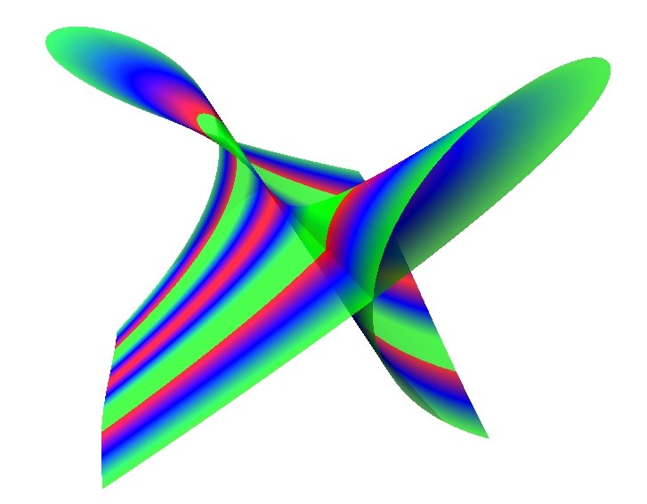
Cayley's ruled cubic has a double line and a singularity called a "unode," which is not a pinch point.
- homogeneous parametrization: [u0u1 : u0u2-u12 : u1u2 : u22]
- homogeneous implicit: x23+x1x2x3-x0x32
- affine implicit: y3+xyz-z2 = 0
- affine cubic parametrization: x=u-v, y=uv, z=u2v, u, v real.
- affine trig parametrization: x=rsin(t)-rcos(t), y=r2sin(t)cos(t), z=r3sin(t)2cos(t), r>=0, 0<=t<=2Pi;
- plot3d([r*sin(t)-r*cos(t), r^2*sin(t)*cos(t), r^3*sin(t)^2*cos(t)], r=0..0.5, t=0..2*Pi, numpoints=1000);
|
POV code
|
The linear transformation which changes the x0 coordinate to x0+x1 gives another view of Cayley's ruled surface.
- homogeneous parametrization: [u0u1+u0u2-u12 : u0u2-u12 : u1u2 : u22]
- homogeneous implicit: x23+x1x2x3-x0x32-x1x32
- affine implicit: y3+xyz-(1+x)z2 = 0
- affine rational parametrization: x=(z2-y3)/(yz-z2), z and y-z nonzero.
- plot3d((z^2-y^3)/(z*y-z^2), y=-2.05..3, z=-2.55..3, view=-5..5, numpoints=1000);
|
10.
Quadric Cases |
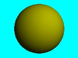 |
Some quadric varieties can also be parametrized by homogeneous quadratic polynomials. For example, the sphere :
- homogeneous parametrization: [u02+u12+u22 : 2u0u2 : 2u0u1: u02-u12-u22]
- homogeneous implicit: x02-x12-x22-x32
- affine implicit: x2+y2+z2-1 = 0
- affine trig parametrization: x=2rsin(t)(1-r2)(1/2), y=2rcos(t)(1-r2)(1/2), z=1-2r2, 0<=r<=1, 0<=t<=2Pi.
- plot3d([2*r*sin(t)*(1-r^2)^(1/2), 2*r*cos(t)*(1-r^2)^(1/2), 1-2*r^2], r=0..1, t=0..2*Pi, numpoints=2500);
For a few more (projectively inequivalent) quadric surfaces
parametrized by quadratic polynomials, see the
page affine
surfaces. |
The main theorem in our paper on Steiner surfaces is that the above
possibilities are essentially the only ones. A surface parametrized by
homogeneous quadratic polynomials is either one of the types 1-9 above
(the parametric map is related to one of the above examples by some
real projective linear change of coordinates), or it is contained in
a quadric
surface, or it is a projection into two or fewer dimensions, so
the image is contained in a plane. The complex classification, which
was previously known, gives fewer equivalence classes: (1,2,3), (4,5),
(6), (7,8), (9), and the quadric and lower-dimensional cases.
POV include file: a .txt file summarizing the implicit equations used in the above graphics, in POV format.
Animation
Here's some POV code for making an animation sequence, and the animated .gif files I assembled using Animation Shop 1.02 by Jasc Software. Click on the  square to load an animated gif
Animations of Steiner Surfaces
|
| 916KB gif
POV scene file
POV ini file
|
The Steiner Roman Surface, rotating around one of its double lines. |
| 215KB gif
POV scene file
POV ini file
|
The Steiner Cross-Cap Surface. The linear transformation(x0,x3) --> (cos(t)x0+sin(t)x3,-sin(t)x0+cos(t)x3)is just a rotation of the (x0,x1,x2,x3) space by angle t, but as the animation cycles, the right edge of the surface meets the "plane at infinity," x0=0, and then re-appears on the left. All the frames show a Type 3 surface; they are equivalent under the linear classification, and look different only because the choice of affine neighborhood is changing. |
| 278KB gif
POV scene file
POV ini file
|
Several different Steiner surfaces. Unlike the above two, which were different views of the same object, in this animation, the object is deforming from one type of Steiner surface to another. The idea is that Types 1, 2, and 3 are stable under perturbation of the parametric equations, and that the Types 4-10 are unstable intermediate cases. In the following equations, the time-dependent quantities are p=cos(t)/sqrt(3) and q=sin(t), 0<=t<=2Pi. The variety is a sphere when p+q=0 (two solutions for t, so two frames), a Type 5 when p=q or p=0 (four frames), and a Roman or Cross-Cap surface for all other values of t. Note the similarity of the homogeneous parametrization with the previous section's equations for Types 5 and 10.
- homogeneous parametrization: [u02+u12+u22 : 2u0u2 : 2u0u1 : 2(pu02-pu12+qu22)]
- affine implicit: (1-2pq-2p2)x4+4pqx2-4p2y2+4(p2-pq)x2y2+4p2y4-2(p+q)x2z+x2z2+y2z2 = 0
Here's some Maple code, showing some of the frames in this loop, parametrized by real numbers e instead of the periodic functions p(t), q(t). Varying the parameter egives a Cross Cap for e < 0, the sphere for e = 0, the Cross Cap again for e between 0 and 2, surface #5 when e = 2, and the Roman Surface for e > 2.
- animate3d([2*r*sin(t)*(1-r^2)^(1/2), 2*r*cos(t)*(1-r^2)^(1/2), -1+2*r^2-r^2*sin(t)^2*e], r=0..1, t=0..2*Pi, e=-2..4, frames=10);
|
| 822KB gif
POV scene file
POV ini file
|
Another deformation of Steiner surfaces. As in the previous animation, the coefficients of the parametric equations depend on another parameter t, 0<=t<=2Pi, and most of the surfaces are either the Type 2, which is not compact in any affine neighborhood, or the Cross Cap, which in this affine neighborhood appears as two components that could be separated by a flat plane. The quantities p=cos(t)/sqrt(3) and q=sin(t) are used again in the following equations. When p=0 (for two frames), the equations define a hyperboloid of two sheets, and when p+q=0 or p-q=0 (for four frames), the surface is a Type 4.
- homogeneous parametrization: [u02+u12-u22 : 2pu12+(q-p)u22 : u1u2 : u0u2]
- affine implicit: 2(pq-p2)y2+(3p-q)xy2-x2y2+(1+2pq-2p2)y4+(p-q)xz2-x2z2+(2-8p2)y2z2+(1-2pq-2p2)z4 = 0
- display3d({animate3d([r^2*sin(t)^2-(1+e)*(r^2-1), r*sin(t)*(r^2-1)^(1/2), r*cos(t)*(r^2-1)^(1/2)], r=1..1.4, t=0..2*Pi, e=-2..1, frames=10), animate3d([-(r^2*sin(t)^2-(1+e)*(r^2+1)), -r*sin(t)*(r^2+1)^(1/2), -r*cos(t)*(r^2+1)^(1/2)], r=0..1, t=0..2*Pi, e=-2..1, frames=10)});
|
The Boy Surface
|
| 557KB gif
POV scene file
POV ini file
|
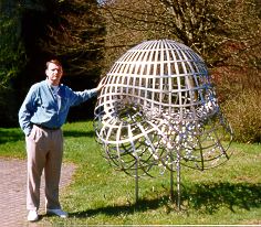 |
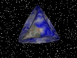
The Boy
Surface is named after Werner Boy, who discovered this immersion
of the real projective plane in three dimensions. It can be realized
as a real algebraic variety of degree six, unlike a Steiner Surface
which has degree at most four. It has a triple point, like the Roman
Surface, but no pinch points. The photo shows
the sculpture
at Oberwolfach. The animation demonstrates F. Apéry's
homotopy, where the equations of the surfaces depend on t,
0<=t<=1. The parametric equations are fourth degree, except that
at t=0, the (u02+u12)
quantity can be canceled from each of the four components, so the t=0
surface is a quadratically parametrized Steiner surface (Type 1). The
implicit equations are sixth degree, but again at t=0, the polynomial
factors into a Steiner quartic and z2. The z2
factor defines the xy-plane, but it is not in the image of the
parametric equations --- it's a locus of extra solutions from the
implicitization, just like the whiskers in the still pictures, and it
is not included in the animation sequence. The image of Apéry's
quartic parametrization of Boy's surface is the t=1 sextic variety,
without any extra implicit solutions. |
- homogeneous parametrization (s=sqrt(2)): [(u02+u12)(u02+u12+u22)+stu1u2(3u02-u12) : (u02+u12)(su02-su12+2u0u2)/3 : 2(u02+u12)(su0u1-u1u2)/3 : (u02+u12)2]
- affine implicit: -24z6 + 48z5 - 32z4 + 64z3/9 - 16y2z2 - 16z2x2 - 81y6t2 - 81x6t2 - (144t2 + 36)y2z2x2 + (72st2 - 72s)y2z2x + (24s - 24st2)z2x3 - (18 + 72t2)y4z2 + (24 - 24t2)y2z3 + (24 - 24t2)z3x2 - (18 + 72t2)z2x4 + (54st3 - 54st)zy5 - (36st + 12st3)z3y3 + (108st - 108st3)x2zy3 + (108st + 36st3)x2z3y + (162st - 162st3)x4zy + 72sy2z3x + 48sy3z2t - 144syz2x2t - 324sy4zxt2 - 216sy2zx3t2 + 36y4zt2 - 243y2x4t2 + 36z4x2t2 - 243y4x2t2 + 36zx4t2 - 24sz3x3 + 36y2z4t2 + 108szx5t2 + 72y2zx2t2= 0
- affine implicit, when t=0: z2(-24z4 + 48z3 - 32z2 - 18y4 + 24y2z - 16y2 + 24zx2 - 16x2 - 18x4 - 36y2x2 + 24sx3 - 24zsx3 + 72zsy2x - 72sy2x + 64z/9) = 0
|
POV code
|
- affine implicit, when t=1: 36zy4 +
36x2z4 + 36x4z -
243x4y2 - 243x2y4 +
36z4y2 + 72x2zy2 -
48sz3y3 + 72sy2z3x -
90y4z2 - 16y2z2 -
16z2x2 - 90z2x4 -
81y6 - 24z6+ 48z5 - 32z4 +
64z3/9 - 81x6 -
180y2z2x2 -
24sz3x3 + 48sy3z2 -
144syz2x2 - 324sy4zx -
216sy2zx3 + 108szx5 +
144sx2z3y = 0
- plot3d([(1+r^2*cos(T)^2)*(sqrt(2)-sqrt(2)*r^2*cos(T)^2+2*r*sin(T)) / (3*(1+r^2*cos(T)^2)*(1+r^2*cos(T)^2+r^2*sin(T)^2) + 3*sqrt(2)*r^2*cos(T)*sin(T)*(3-r^2*cos(T)^2)), 2*(1+r^2*cos(T)^2)*(sqrt(2)*r*cos(T) - r^2*cos(T)*sin(T)) / (3*(1+r^2*cos(T)^2)*(1+r^2*cos(T)^2+r^2*sin(T)^2) + 3*sqrt(2)*r^2*cos(T)*sin(T)*(3-r^2*cos(T)^2)), (1+r^2*cos(T)^2)^2 / ((1+r^2*cos(T)^2)*(1+r^2*cos(T)^2+r^2*sin(T)^2) + sqrt(2)*r^2*cos(T)*sin(T)*(3-r^2*cos(T)^2))], r=0..10, T=0..2*Pi, numpoints=2000);
|
Web Sites
| Links related to Steiner surfaces :
Software:
Books:
Academic papers, abstracts, etc.:
- A. Adler, "cubic
surfaces" newsgroup post
- F. Aries, E. Briand, C. Bruchou, "Some covariants related to Steiner surfaces"
- D. Breen, publications
- A. de Cusatis Jr., L. Henrique de Figueiredo, M. Gattass, "Interval methods..." Proc. SIBGRAPI'99 reprint
- H. Farran, M. do Rosario Pinto, S. Robertson, "Symmetric Models..." BzA&G reprint
- F. Halter-Koch and G. Lettl, "Polynomial parametrization of systems of Diophantine equations"
- S. Klimenko, I. Nikitin, V. Burkin, Visualization Proceedings article
- R. Krasauskas, Shape of toric surfaces
- J. Peters, U. Reif, "Quadratic Surfaces..." CAGD reprint
- C. Rourke, B. Sanderson, "The Compression Theorem" reprint
- J. Schicho, "Multiple Conical Surfaces" BzA&G reprint
- H.-P. Schröcker, "A Family of Conics and Three Special Ruled Surfaces" BzA&G reprint
- T. Sederberg, publications
- S. Zube, publications
|
Links to pictures of Steiner surfaces:
- The Geometry Center
- J. Baez, Klein's Quartic
- P. Bourke, Geometry
- S. Endraß, Surf gallery
- Z. Fiedorowicz, (Topological) Classification of Surfaces
- P. Fur Mat, Approximate Cat
- W. Gu, Curves and Surfaces library
- H. Hauser, Singularities pictures and animation
- H. Havlicek, Veronese varieties
- B. Hunt, Algebraic
Surfaces
- A. Lipson, Mathematical Lego Sculptures
- J.-L. Maltret, Mathématiques et Informatique Graphique
- T. Nordstrand, surface gallery, in particular, ray-traced Steiner surfaces of types 1, 2, 3, 4.
- R. Palais, 3-D XplorMath
- S. Popescu, Algebraic Topology
- C. Séquin, graphics and sculpture
- J. Tunnell,
Rutgers Math
535
- M. Williams, Isosurface Tutorial
- UIUC display case with Plaster Models
- NYIT Computer Graphics Lab pictures
More Links
- Adam
Coffman, Art
Schwartz, C. Stanton, 1996 article, The
algebra and geometry of Steiner and other quadratically parametrizable
surfaces
- Google Scholar Citations for the CAGD article
- Google Scholar Citations for this Steiner Surfaces web page
- Google Books about Steiner surfaces
- ACM Digital Library page
- A. Coffman, A Classification of Quadratically Parametrized
Maps of the Real Projective Plane, B.S. Honors Thesis,
University of Michigan, Ann Arbor, 1991.
- Re-typeset, added update sections, and posted online in
2018: 37 pages + 10 Figures.
- A. Schwartz and C. Stanton, Classification of Steiner Surfaces, unpublished notes from 1988, available from me on request.
- More papers by Adam Coffman
|
Back to Adam Coffman's page


 916KB gif
 215KB gif
 278KB gif
 822KB gif
 557KB gif