Surfaces and horizontal tangents

One way to represent the surface is in the x,y,z real coordinate system, as the graph of a function

Another way to represent the surface is in the (z₁,z₂) coordinate system, where z₁ and z₂ are both complex numbers: z₁=x₁+iy₁ and z₂=x₂+iy₂. In the following pictures, the surface can be plotted as a graph:

The blue formulas give h(z1), followed by f(x,y)

Elliptic The critical point at the center of the dot is a local minimum value. 0 < γ < 1/2 Maple worksheet POV scene file

Hyperbolic The critical point is a saddle point at the center of the X shape. 1/2 < γ < ∞ Maple worksheet POV scene file

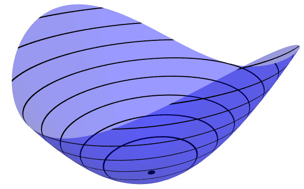
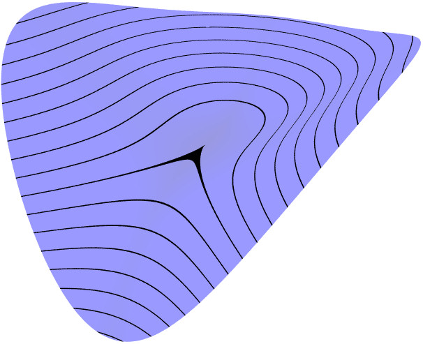
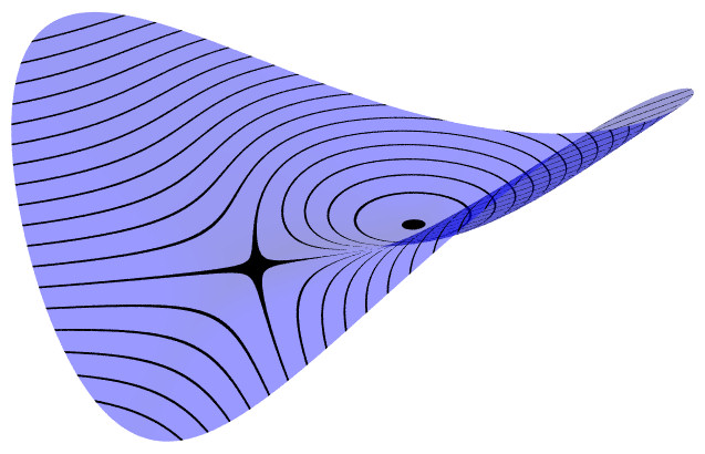
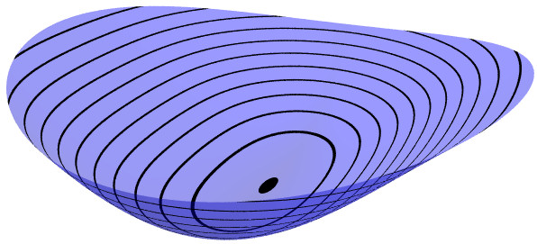
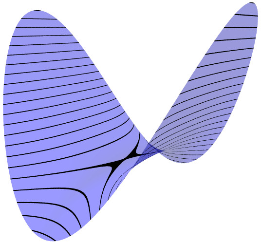
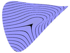
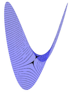
Cubic Parabolic The level set through the critical point has a cusp shape. This kind of critical point is "unstable," in the sense that small changes in the function can result in a surface with different kinds of critical points, as the following two pictures show. Maple worksheet POV scene file γ = 1/2

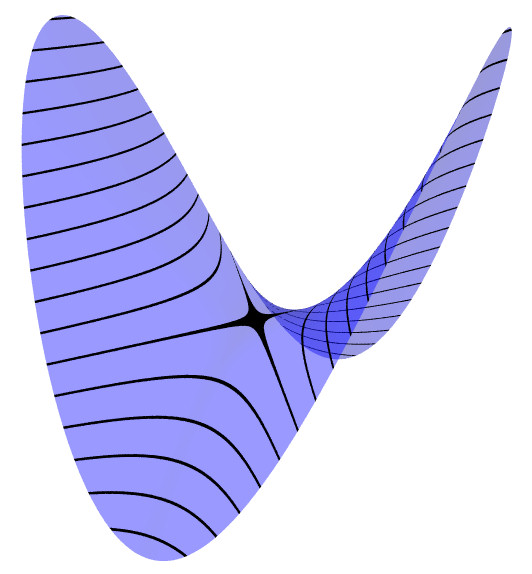
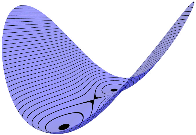
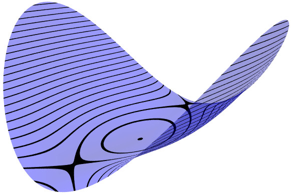
Deformation of Cubic Parabolic into Elliptic/Hyperbolic pair Adding a linear term with coefficient t < 0 deforms the surface with an unstable parabolic critical point into a surface with a pair of stable critical points, one elliptic and one hyperbolic. Maple worksheet POV scene file

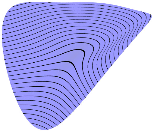
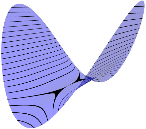
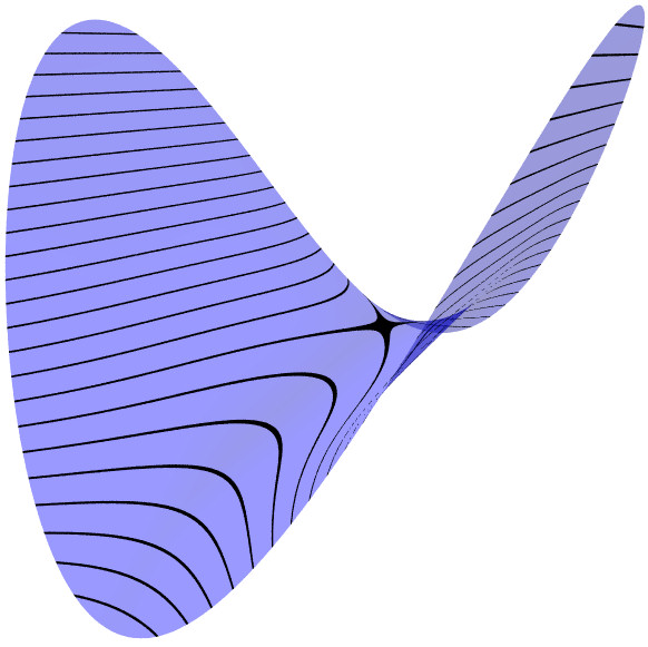
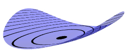
Deformation of Cubic Parabolic into surface without critical points Using the same formula as above, but with linear coefficient t >0, results in a surface with no critical points. This can be understood as a "cancellation" phenomenon, where t is a time parameter, and the elliptic/hyperbolic points move toward each other as t increases, collide at t=0 to form a parabolic point, and then disappear as t becomes positive. Maple worksheet POV scene file

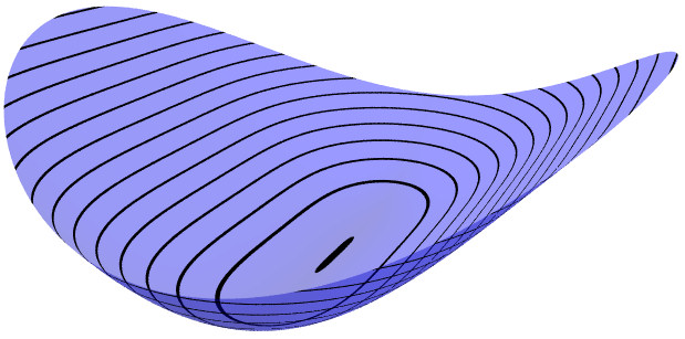
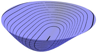
There are two types of quartic (degree 4) surfaces with a parabolic critical point; for lack of better terminology, they are labeled type (I) and type (II). Quartic Parabolic (I) This surface also has a critical point which is a local minimum. In the picture, the surface is more flat in the y direction than the x direction, and the critical point is in the center of the long black dot. The surface is defined by a quartic (degree 4) equation and is unstable under deformations, as the following three pictures show. Maple worksheet POV scene file

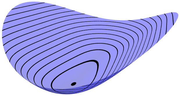
Deformation of Quartic Parabolic (I) into Elliptic Adding a linear term with coefficient t1 < 0 or t1 > 0 gives a stable elliptic critical point. Maple worksheet POV scene file

Deformation of Quartic Parabolic (I) into Elliptic Adding quadratic terms with coefficient t2 < 0 also gives a stable elliptic critical point. Maple worksheet POV scene file

Deformation of Quartic Parabolic (I) into two Elliptic + one Hyperbolic Adding the same quadratic terms with coefficient t2 > 0 gives three stable critical points. Maple worksheet POV scene file

Quartic Parabolic (II) This surface has a critical point where surface is more flat in the y direction than the x direction, and the level set through the critical point is a self-tangent curve, instead of an X shape like the stable saddle point. Maple worksheet POV scene file

Deformation of Quartic Parabolic (II) into Hyperbolic Adding a linear term with coefficient t1 < 0 or t1 > 0 gives a stable hyperbolic critical point. Maple worksheet POV scene file

Deformation of Quartic Parabolic (II) into Hyperbolic Adding quadratic terms with coefficient t2 > 0 also gives a stable hyperbolic critical point. Maple worksheet POV scene file

Deformation of Quartic Parabolic (II) into two Hyperbolic + one Elliptic Adding the same quadratic terms with coefficient t2 < 0 gives three stable critical points. Maple worksheet POV scene file

Animations Click on the small image to see an animation

150KB gif POV scene file POV ini file A surface with an elliptic point, γ = 1/4, can be deformed using a time parameter t, by replacing γ with γ + t, and the surface will still be elliptic for t close to 0. In the animation, t varies between -0.2 and +0.2, so the coefficient γ varies between 0.05 (almost circular cross sections) to 0.45 (almost a parabolic cylinder). The (black) level curves are always ellipses although this implicit equation also has some cubic terms. The "deflating ellipsoid" animation on the graphics gallery page also demonstrates this type of deformation.

250KB gif POV scene file POV ini file This is the deformation of a cubic parabolic point, as described above, so sometimes there is a pair of critical points, and sometimes there is no critical point.

596KB gif POV scene file POV ini file This is a deformation of the quartic parabolic point, Type I, as described above. There is a two-dimensional parameter space (coordinates t1, t2), so to get an animation depending on the time parameter T only, let t1, t2 follow an elliptical path (green) in the parameter space, so that at the start time T=0, the parameters are at the origin, so the surface has the quartic parabolic normal form. As time passes, the parameters move around the ellipse - when (t1, t2) is below the (red) discriminant curve, the surface has exactly one elliptic point, when (t1, t2) is a point on the curve but not at the cusp, the surface has an elliptic point and a cubic parabolic point, and when (t1, t2) is a point above the curve, the surface has two elliptic points and one hyperbolic point.

318KB gif POV scene file POV ini file This is a deformation of the quartic parabolic point, Type II, as described above. There is a two-dimensional parameter space (coordinates t1, t2), so to get an animation depending on the time parameter T only, let t1, t2 follow an elliptical path (green) in the parameter space, so that at the start time T=0, the parameters are at the origin, so the surface has the quartic parabolic normal form. As time passes, the parameters move around the ellipse - when (t1, t2) is above the (red) discriminant curve, the surface has exactly one hyperbolic point, when (t1, t2) is a point on the curve but not at the cusp, the surface has a hyperbolic point and a cubic parabolic point, and when (t1, t2) is a point below the curve, the surface has two hyperbolic points and one elliptic point.